How to do linear regression in Excel using LINEST
24 July 2016
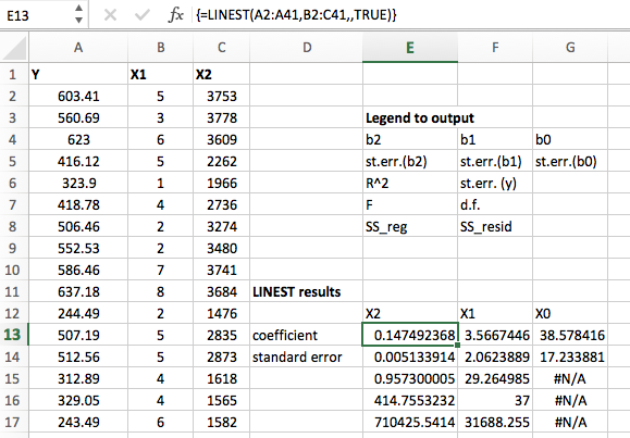
My friend was asking me for help with running linear regression in Excel. I had never tried this before, since I normally would use R for this purpose, but I finally figured it out. While I do not recommend using Excel for regression, if you have no choice maybe these instructions may be helpful. Here is a screenshot of what it looks like:
Excel Approach
Let’s say we have a data table with columns Y,X1,X2. Y is the outcome we want to predict, such as dollars spent on food. X1 and X2 are predictor variables, such as family size and income. To run linear regression, use the LINEST command. This command is unnecessarily complicated. Suppose the data table occupies cells A1:C100 such that the first row are the column names and the actual values are in A2:C100. Suppose the outcome variable Y is in the first column (column A) and the predictor variables X1 and X2 are in columns B and C respectively.
- Find a blank space in the sheet and highlight a block of cells, the block should have a height of 5 cells and a width of however many variables you have (in this example, 3 variables: one intercept term plus two predictor variables).
- Go to the formula bar and type the LINEST command, for example
=LINEST(A2:A100,B2:C100,,TRUE). The first argument is the outcome variable data points (Y). The second argument is the array of predictor variables (X1,X2). The third argument should be left empty as setting it can force the model to not use an intercept, which is almost always a bad idea. Finally, the TRUE part at the last position tells excel to return summary statistics for the model fit. - Don’t push enter or hit equals! Instead, you need to make it an array formula by holding down control and shift then hitting enter. If this works, the block of cells should fill up with a bunch of numbers. If it didn’t work, there will be #VALUE everywhere. The secret key combination for array formula may be different for older versions of excel, or for macs. Try searching for array formula to find the right version if you get stuck. Note that it is OK for there to be #N/A values in the lower right block of the output. Only the first two columns will have values all the way down. Note that if you click on the formula block again it will have braces around the formula like this
{=LINEST(....)}. That is something Excel does automatically to indicate array formulas. You shouldn’t have to type the braces. - The interpretation of the output is in the REVERSE order from the way the variables are stored in the data. So if you have Y,X1,X2 in the data table, the model output will be coefficients and standard errors for X2,X1, and then the intercept term.
- The first row of the block output are the regression coefficients, also known as the effects of the predictor variables on the response. The second row holds the corresponding standard errors, which can be used to construct confidence intervals or do tests of significance. The third row is the R^2 value and the standard error of the response variable (Y). The fourth row is the F statistic and the degrees of freedom. This can be used for testing the significance of the model as a whole. Finally in the fifth row are the regression sum of squares and the residual sum of squares, which are quantities used in computing the R^2 value and F statistic. They are rarely interpreted directly.
Easier Approach using R
Save the sheet as a CSV file and open R. Use the following commands to get the same result.
dat<-read.csv("name_of_data_file.csv")
colnames(dat) <- c("Y","X1","X2")
mod1<- lm(Y ~ X1 + X2, data=dat)
summary(mod1)